习题3 - 图像恢复实验内容 图像是一种非常常见的信息载体,但是在图像的获取、传输、存储的过程中可能由于各种原因使得图像受到噪声的影响——称为图像退化。图像复原就是重建退化的图像,使其最大限度恢复景物原貌的处理。如何去除噪声的影响,恢复图像原本的信息是计算机视觉中的重要研究问题。
常见的图像恢复算法有基于空间域的中值滤波、基于小波域的小波去噪、基于偏微分方程的非线性扩散滤波等,在本次实验中,📌我们要对图像添加噪声,并对添加噪声的图像进行基于模型的去噪 。
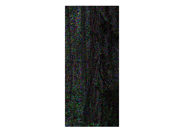
实验要求 A. 生成受损图像。
a) 受损图像是由原始图像添加了不同噪声遮罩(noise masks)得到的。
b) 噪声遮罩仅包含 {0,1} 值。对原图的噪声遮罩的可以每行分别用 0.8/0.4/0.6 的噪声比率产生的,即噪声遮罩每个通道每行 80%/40%/60% 的像素值为 0,其他为 1。
B. 使用模型,进行图像恢复。
C. 评估误差为所有恢复图像与原始图像的 2-范数之和,此误差越小越好,其他评估方式包括 Cosine 相似度以及 SSIM 相似度。
D. 提交程序报告,请在本地编辑并命名为『程序报告.docx』或者 『程序报告.pdf』后, 上传到左侧文件列表中。
实验环境 可以使用基于Python的 OpenCV 库进行图像相关处理,使用 Numpy 库进行相关数值运算。
参考资料 OpenCV:https://opencv-python-tutroals.readthedocs.io/en/latest/py_tutorials/py_tutorials.html
Numpy:https://www.numpy.org/
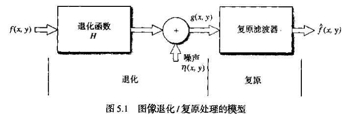
设原始图像 f ( x , y ) , f(x, y), f ( x , y ) ,
g ( x , y ) = H [ f ( x , y ) ] + η ( x , y ) g(x, y)=H[f(x, y)]+\eta(x, y)
g ( x , y ) = H [ f ( x , y ) ] + η ( x , y )
其中 H H H η ( x , y ) \eta(x, y) η ( x , y ) f ^ ( x , y ) , \hat{f}(x, y), f ^ ( x , y ) ,
g ( x , y ) = h ( x , y ) ∗ f ( x , y ) + η ( x , y ) g(x, y)=h(x, y) * f(x, y)+\eta(x, y)
g ( x , y ) = h ( x , y ) ∗ f ( x , y ) + η ( x , y )
进行傅立叶变换, 有
G ( u , v ) = H ( u , v ) F ( u , v ) + N ( u , v ) G(u, v)=H(u, v) F(u, v)+N(u, v)
G ( u , v ) = H ( u , v ) F ( u , v ) + N ( u , v )
1. 图像增强与图像复原的区别 图像增强的目的是消除噪声,显现那些被模糊了的细节或简单地突出一幅图像中读者感兴趣的特征,不考虑图像质量下降的原因。图像复原是利用退化现象的某种先验知识 ,建立退化现象的数学模型,再根据模型进行反向的推演运算,以恢复原来的景物图像。因而,图像复原可以理解为图像降质过程的反向过程。建立图像复原的反向过程的数学模型,就是图像复原的主要任务。经过反向过程的数学模型的运算,要想恢复全真的景物图像比较困难。所以, 图像复原本身往往需要有一个质量标准, 即衡量接近全真景物图像的程度,或者说,对原图像的估计是否到达最佳的程度。
2. 噪声模型: 噪声主要来源于图像的获取和传输过程。
(1)图像传感器的工作情况受各种因素的影响,如图像获取中的环境条件和传感器元器件自身的质量。
(2)图像在传输过程中主要由于所用传输信道被干扰而受到噪声污染。
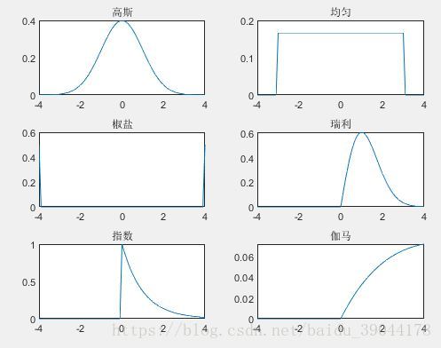
**噪声种类:**高斯噪声、瑞利噪声、伽马噪声、指数噪声、均匀分布噪声、脉冲噪声(椒盐噪声)
1 2 3 4 5 6 7 8 9 10 11 12 13 14 15 16 17 18 19 20 21 22 23 24 25 x=-4 :.1 :4 ; subplot(321 ) Y1=show_noise_pdf('gaussian' ,x,0 ,1 ); plot(x,Y1); title('高斯' ); subplot(322 ) Y2=show_noise_pdf('uniform' ,x,-3 ,3 ); plot(x,Y2); title('均匀' ); subplot(323 ) Y3=show_noise_pdf('salt & pepper' ,x); plot(x,Y3); title('椒盐' ); subplot(324 ) Y4=show_noise_pdf('rayleigh' ,x,1 ); plot(x,Y4); title('瑞利' ); subplot(325 ) Y5=show_noise_pdf('exp' ,x,1 ); plot(x,Y5); title('指数' ); subplot(326 ) Y6=show_noise_pdf('gamma' ,x,2 ,5 ); plot(x,Y6); title('伽马' );
概率密度函数:p ( z ) = 1 2 π σ e − ( z − μ ) 2 2 σ 2 p(z)=\frac{1}{\sqrt{2πσ}}e^{−\frac{(z−μ)^2}{2σ^2}} p ( z ) = 2 π σ 1 e − 2 σ 2 ( z − μ ) 2 μ μ μ σ 2 σ^2 σ 2
高斯噪声是一个均值为 0 方差为 $σ_n^2 $的正态分布,是一个加性噪声(在原图的基础上加上噪声即为加噪后的图象)。但要正确地给图片添加高斯噪声,还要取决于程序中读入图片的数据格式。
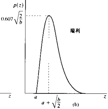
概率密度函数: p ( z ) = { 2 b ( z − a ) e − ( z − a ) 2 / b , z ≥ a 0 , z < a 均值: μ = a + π b / 4 方差: σ 2 = b ( 4 − π ) 4 \begin{aligned}
&\text { 概率密度函数: }\\
&p(z)=\left\{\begin{array}{ll}
\frac{2}{b}(z-a) e^{-(z-a)^{2} / b}, & z \geq a \\
0, & z<a
\end{array}\right.\\
&\text { 均值: } \mu=a+\sqrt{\pi b} / 4\\
&\text { 方差: } \sigma^{2}=\frac{b(4-\pi)}{4}
\end{aligned}
概率密度函数: p ( z ) = { b 2 ( z − a ) e − ( z − a ) 2 / b , 0 , z ≥ a z < a 均值: μ = a + π b / 4 方差 : σ 2 = 4 b ( 4 − π )
曲线:
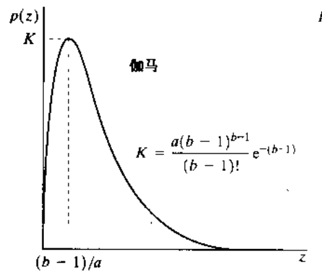
概率密度函数: p ( z ) = { a b z ( b − 1 ) ( b − 1 ) ! e − a z , z ≥ 0 0 , z < 0 均值: μ = b a 方差: σ 2 = b a 2 \begin{aligned}
&\text { 概率密度函数: }\\
&p(z)=\left\{\begin{array}{ll}
\frac{a^{b} z^{(b-1)}}{(b-1) !} e^{-a z}, & z \geq 0 \\
0, & z<0
\end{array}\right.\\
&\text { 均值: } \mu=\frac{b}{a}\\
&\text { 方差: } \sigma^{2}=\frac{b}{a^{2}}
\end{aligned}
概率密度函数: p ( z ) = { ( b − 1 ) ! a b z ( b − 1 ) e − a z , 0 , z ≥ 0 z < 0 均值: μ = a b 方差: σ 2 = a 2 b
曲线:
概率密度函数: p ( z ) = { a e − a z , z ≥ 0 0 , z < 0 均值: μ = 1 a 方差: σ 2 = 1 a 2 \begin{aligned}
&\text { 概率密度函数: }\\
&p(z)=\left\{\begin{array}{ll}
a e^{-a z}, & z \geq 0 \\
0, & z<0
\end{array}\right.\\
&\text { 均值: } \mu=\frac{1}{a}\\
&\text { 方差: } \sigma^{2}=\frac{1}{a^{2}}
\end{aligned}
概率密度函数: p ( z ) = { a e − a z , 0 , z ≥ 0 z < 0 均值 : μ = a 1 方差: σ 2 = a 2 1
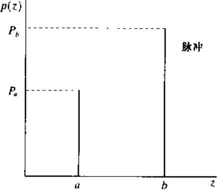
概率密度函数: 双极脉冲口声 p ( z ) = { P a , z = a P b , z = b 0 , 其他 p(z)=\left\{\begin{array}{ll}P_{a}, & z=a \\ P_{b}, & z=b \\ 0, & \text { 其他 }\end{array}\right. p ( z ) = ⎩ ⎨ ⎧ P a , P b , 0 , z = a z = b 其他
3. 空间滤波
图像滤波器又叫做掩模 、核 、模板 或窗口 ,是与原图像的子图像有相同维数的子图像,滤波器子图像中的值是系数值 ,不是像素值,滤波器的处理结果是子图像中心位置像素值等于被掩住位置的像素值与滤波器中系数的点积和 。
无论是平均平滑还是高斯平滑,在处理图像噪声时,都或多或少会对图片产生一定的模糊 ,损失部分信息。较为理想的情况,是可以选择性地进行滤波,只在噪声区域进行平滑,而在无噪声区域不进行平滑,将模糊的影响降到最低,这就是自适应性滤波的思想。通常噪声的存在,可能会使得附近邻域内,极值的上下差距较大,或者是方差较大,我们可以设置一定的阈值来判断该点是否需要进行平滑。不过这个不是该章节的内容。
不同的滤波器在处理不同类型的噪声是效果不同,对于线性平滑滤波,在处理像素邻域内的噪声点时,噪声或多或少都会影响该点的像素值计算(以高斯平滑为例,距离近则影响大,距离远则影响小,与距离的平方呈反比);但是中值滤波通常可以将噪声点直接忽略掉。同时,中值滤波在降噪的同时引起的模糊效应较低。中值滤波的一种典型应用,就是用来消除椒盐(salt & pepper)噪声。
**空间滤波器种类:**均值滤波器(适于高斯噪声)、统计排序滤波器(适于椒盐噪声)、自适应局部噪声消除滤波器(适于所有噪声)、自适应中值滤波器(适于椒盐噪声)。
空域滤波器分为平滑滤波器 和锐化滤波器 ,平滑滤波用积分 实现,锐化滤波用微分 实现
算术均值滤波器 描述: f ^ ( x , y ) = ∑ ( s , t ) ∈ S x y g ( s , t ) \hat{f}(x, y)=\sum_{(s, t) \in S_{x y}} g(s, t) f ^ ( x , y ) = ∑ ( s , t ) ∈ S x y g ( s , t )
几何均值滤波器 描述: f ^ ( x , y ) = [ ∏ ( s , t ) ∈ S x y g ( s , t ) ] \hat{f}(x, y)=\left[\prod_{(s, t) \in S_{x y}} g(s, t)\right] f ^ ( x , y ) = [ ∏ ( s , t ) ∈ S x y g ( s , t ) ]
谐波均值滤波器 描述: f ^ ( x , y ) = m n ∑ ( z , y ) ∈ S z y 1 g ( s , t ) \hat{f}(x, y)=\frac{m n}{\sum_{(z, y) \in S_{z y}} \frac{1}{g(s, t)}} f ^ ( x , y ) = ∑ ( z , y ) ∈ S z y g ( s , t ) 1 m n
结果:谐波均值滤波器对于“盐”噪声效果更好,但是不适用于“胡椒”噪声。
逆谐波均值滤波器
高斯滤波
GaussianBlur, k窗口值都是奇数,如3、5、7,越靠近中心的权重越大。整个高斯核跟图像窗口做卷积后取其值
中值滤波器f ^ ( x , y ) = median ( s , t ) ∈ S x y { g ( s , t ) } \hat{f}(x, y)=\operatorname{median}_{(s, t) \in S_{x y}\{g(s, t)\}} f ^ ( x , y ) = m e d i a n ( s , t ) ∈ S x y { g ( s , t ) } 统计排序滤波器 ,是以该点为中心的的邻域内的所有像素的统计排序中值作为该点的响应;而平滑就是加权平均数作为响应,概念上有一定差别。
视频讲解:https://www.bilibili.com/video/BV1fQ4y1N7EP?from=search&seid=11848827709822211739
最大值滤波器 描述: f ^ ( x , y ) = max ( s , t ) ∈ S z y { g ( s , t ) } \hat{f}(x, y)=\max _{(s, t) \in S_{z y}}\{g(s, t)\} f ^ ( x , y ) = max ( s , t ) ∈ S z y { g ( s , t ) }
最小值滤波器 描述: f ^ ( x , y ) = min ( s , t ) ∈ S x y { g ( s , t ) } \hat{f}(x, y)=\min _{(s, t) \in S_{x y}}\{g(s, t)\} f ^ ( x , y ) = min ( s , t ) ∈ S x y { g ( s , t ) }
中点滤波器 描述: f ^ ( x , y ) = [ max ( s , t ) ∈ S x y { g ( s , t ) } + min ( s , t ) ∈ S x y { g ( s , t ) } ] \hat{f}(x, y)=\left[\max _{(s, t) \in S_{x y}}\{g(s, t)\}+\min _{(s, t) \in S_{x y}}\{g(s, t)\}\right] f ^ ( x , y ) = [ max ( s , t ) ∈ S x y { g ( s , t ) } + min ( s , t ) ∈ S x y { g ( s , t ) } ]
修正后的阿尔法均值滤波體 描述: f ^ ( x , y ) = 1 m n ∑ ( s , t ) ∈ S x y { g r ( s , t ) } \hat{f}(x, y)=\frac{1}{m n} \sum_{(s, t) \in S_{x y}}\left\{g_{r}(s, t)\right\} f ^ ( x , y ) = m n 1 ∑ ( s , t ) ∈ S x y { g r ( s , t ) } S x y S_{xy} S x y
自适应滤波器的行为变化基于由m*n矩形窗口Sxy定义的区域内图像的统计特性,它的性能要明显优于前面介绍的滤波器,代价是滤波器的复杂度。
自适应、局部噪声消除滤波器f ^ ( x , y ) = g ( x , y ) − σ η 2 σ L 2 [ g ( x , y ) − m L ] \hat{f}(x, y)=g(x, y)-\frac{\sigma_{\eta}^{2}}{\sigma_{L}^{2}}\left[g(x, y)-m_{L}\right] f ^ ( x , y ) = g ( x , y ) − σ L 2 σ η 2 [ g ( x , y ) − m L ] σ η 2 , g ( x , y ) \sigma_{\eta}^{2}, g(x, y) σ η 2 , g ( x , y ) m L , m_{L}, m L , σ L 2 , \sigma_{L}^{2}, σ L 2 , σ η 2 \sigma_{\eta}^{2} σ η 2 g ( x , y ) g(x, y) g ( x , y ) σ η 2 \sigma_{\eta}^{2} σ η 2 g ( x , y ) g(x, y) g ( x , y ) σ η 2 \sigma_{\eta}^{2} σ η 2
自适应中值滤波器
Zmin=Sxy中灰度值的最小值
Zmax=Sxy中灰度值的最大值
Zmed=Sxy中灰度值的中间值
Zxy=在坐标(x,y)上的灰度值
Smax=Sxy允许的最大尺寸
from: https://blog.csdn.net/xdmdth/article/details/46889091?utm_medium=distribute.pc_relevant.none-task-blog-BlogCommendFromBaidu-3.control&depth_1-utm_source=distribute.pc_relevant.none-task-blog-BlogCommendFromBaidu-3.control
1
2
3
4
5
6
7
8
9
10
11
12
13
14
15
16
17
18
19
class NoiseGenerator : @staticmethod def add_pulse_noise (im, noise_ratios=0.3 ) : """ 给图像增加脉冲噪声 脉冲噪声:噪声点只有两种情况,全黑or全白,因此又称为椒盐噪声 :param im: 待处理的图像 :param noise_ratios: 噪声比 :return: """ h, w = im.shape[0 :2 ] p_size = h * w for r in range(int(p_size * noise_ratios)): rand_h = random.randint(0 , h - 1 ) rand_w = random.randint(0 , w - 1 ) im[rand_h, rand_w, :] = np.array([0 , 0 , 0 ]) if random.random() < 0.5 else np.array([255 , 255 , 255 ]) return im
1
2
3
4
5
6
7
8
9
10
11
12
13
14
15
16
17
18
19
20
21
22
23
24
25
26
27
28
29
30
31
32
33
34
35
36
37
class NoiseGenerator : @classmethod def _normalization (cls, image) : """ 将数据线性归一化 :param image: 图片矩阵,一般是np.array 类型 :return: 将归一化后的数据,在(0,1)之间 """ info = np.iinfo(image.dtype) return image.astype(np.double) / info.max @staticmethod def add_gaussian_noise (im, mean=0 , var=0.005 ) : """ 添加高斯噪声 :param im: :param mean: 均值 :param var: 方差 :return: """ image = NoiseGenerator._normalization(im) noise = np.random.normal(mean, var ** 0.5 , image.shape) noised_im = image + noise def clip_img (noised_im) : """ 将值限制在(-1或0, 1)间,然后乘255恢复 :param noised_im: 加了噪声的图片 :return: clip过的图片 """ "" low_clip = -1. if noised_im.min() < 0 else 0. out_im = np.clip(noised_im, low_clip, 1.0 ) out_im = np.uint8(out_im * 255 ) return out_im return clip_img(noised_im)
▲这边肯定有人会好奇out_im = np.uint8(out_im * 255)并不是将其转换到(0, 255),而是(-255, 255)。 解释一下:——注意这边的np.uint8可以看到这边的数据类型就是8位int,所以范围是0-255,因此即使num=-55,那么计算的结果其实是201; num=-1,结果其实是255。
法二:skimage
1
2
3
4
5
6
7
8
9
10
11
12
13
14
15
16
17
from matplotlib import pyplot as pltfrom skimage import ioimport skimageimport pylabimpath = "000001.jpg" image = io.imread(impath) img1 = image / 255.00 img2 = skimage.util.random_noise(image,mode='gaussian' ,seed=None ,clip=True ) plt.figure(1 ) plt.subplot(121 ) plt.imshow(img1) plt.title("Origin picture" ) plt.subplot(122 ) plt.imshow(img2) plt.title("Add Gaussian noise" ) pylab.show() plt.savefig("noise_image.jpg" )
注意到:增加高斯噪声还可以用图像三方库完成的:skimage.util.random_noise(image,mode ='gaussian',seed=None,clip=True)
skimage即是Scikit-Image。基于python脚本语言开发的数字图片处理包,比如PIL,Pillow, opencv, scikit-image等。
PIL和Pillow只提供最基础的数字图像处理,功能有限;opencv实际上是一个c++库,只是提供了python接口,更新速度非常慢。scikit-image是基于scipy 的一款图像处理包,它将图片作为numpy数组进行处理,正好与matlab一样,因此,我们最终选择scikit-image进行数字图像处理。
skimage包的全称是scikit-image SciKit (toolkit for SciPy) ,它对scipy.ndimage进行了扩展,提供了更多的图片处理功能。它是由python语言编写的,由scipy 社区开发和维护。skimage包由许多的子模块组成,各个子模块提供不同的功能。
子模块名称
主要实现功能
io
读取、保存和显示图片或视频
data
提供一些测试图片和样本数据
color
颜色空间变换
filters
图像增强、边缘检测、排序滤波器、自动阈值等
draw
操作于numpy数组上的基本图形绘制,包括线条、矩形、圆和文本等
transform
几何变换或其它变换,如旋转、拉伸和拉东变换等
morphology
形态学操作,如开闭运算、骨架提取等
exposure
图片强度调整,如亮度调整、直方图均衡等
feature
特征检测与提取等
measure
图像属性的测量,如相似性或等高线等
segmentation
图像分割
restoration
图像恢复
util
通用函数
本质上是低通滤波器,输出图像的每个像素点是原图像上对应像素点与周围像素点的加权和。
即用高斯分布权值矩阵与原始图像矩阵做卷积运算。
https://blog.csdn.net/qq_37995260/article/details/100351153
Python给图像添加噪声具体操作
1 2 3 4 5 6 7 8 9 10 11 12 13 14 15 16 17 18 19 20 21 22 23 24 25 26 27 28 29 30 31 32 33 34 35 36 37 38 39 40 41 42 43 44 45 46 def noise_mask_image (img, noise_ratio) : """ 根据题目要求生成受损图片 :param img: 图像矩阵,一般为 np.ndarray :param noise_ratio: 噪声比率,可能值是0.4/0.6/0.8 :return: noise_img 受损图片, 图像矩阵值 0-1 之间,数据类型为 np.array, 数据类型对象 (dtype): np.double, 图像形状:(height,width,channel),通道(channel) 顺序为RGB """ noise_img = None mask = np.random.choice([0 , 1 ], size=(img.shape[0 ],img.shape[1 ],img.shape[2 ]), p = [noise_ratio, 1 - noise_ratio]) noise_img = mask * img return noise_img def noise_mask_image (img, noise_ratio) : """ 根据题目要求生成受损图片 :param img: 图像矩阵,一般为 np.ndarray :param noise_ratio: 噪声比率,可能值是0.4/0.6/0.8 :return: noise_img 受损图片, 图像矩阵值 0-1 之间,数据类型为 np.array, 数据类型对象 (dtype): np.double, 图像形状:(height,width,channel),通道(channel) 顺序为RGB """ noise_img = None import random from copy import deepcopy noise_img = deepcopy(img) h, w = img.shape[: 2 ] for dh in range(h): cols = range(w) mask_indexes = random.sample(cols, int(w * noise_ratio)) pixel_list = [0 if i in mask_indexes else 1 for i in cols] for c in cols: noise_img[dh, c, :] = noise_img[dh, c, :] * pixel_list[c] noise_img = np.array(noise_img, dtype='double' ) return noise_img
Python的random操作
1
2
3
4
5
6
7
8
9
10
11
12
13
14
15
16
17
18
19
20
21
22
23
24
25
26
27
28
29
30
31
32
33
34
35
36
37
38
39
40
41
42
43
44
45
46
47
48
49
50
51
52
53
54
55
56
57
58
59
60
61
from PIL import Imageimport numpy as npdef AddNoise (src, dst, probility=0.05 ) : """ salt_pepper增加噪声 :param src: :param dst: :param probility: :return: """ imarray = np.array(Image.open(src)) height, width = imarray.shape[:2 ] for i in range(height): for j in range(width): if np.random.random(1 ) < probility: if np.random.random(1 ) < 0.5 : imarray[i, j, :] = 0 else : imarray[i, j, :] = 255 new_im = Image.fromarray(imarray) new_im.save(dst) def MedianFilter (src, dst, k=3 , padding=None) : """ 中值滤波 :param src: :param dst: :param k: 过滤器核大小 :param padding: :return: """ imarray = np.array(Image.open(src)) height, width, channels = imarray.shape if not padding: edge = int((k - 1 ) / 2 ) if height - 1 - edge <= edge or width - 1 - edge <= edge: print("The parameter k is to large." ) return None new_arr = np.zeros((height, width, 3 ), dtype="uint8" ) for i in range(height): for j in range(width): for c in range(channels): if i <= edge - 1 or i >= height - 1 - edge or j <= edge - 1 or j >= width - edge - 1 : new_arr[i, j, c] = imarray[i, j, c] else : new_arr[i, j, c] = np.median(imarray[i - edge:i + edge + 1 , j - edge:j + edge + 1 , c]) new_im = Image.fromarray(new_arr) new_im.save(dst) if __name__ == '__main__' : gray_girl = "A.png" tar = "A_noised.png" AddNoise(gray_girl, tar) src = "A_noised.png" dst = "A_repaired.png" MedianFilter(src, dst)
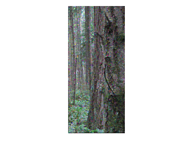
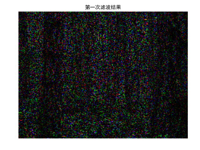
下图是k=3是的改进后的中值滤波策略的结果,可以看到图像的清晰度得到了较大的保留,噪声的数量就相对也残留的比较多。从中可以看到,二者之间有此消彼长的关系。至于为什么还有这么多的椒盐噪声,原因是因为我们添加噪声的代码中设置的概率太高了,导致图像中的椒盐噪声数量非常多,在小区域内有可能有许多的噪声点,导致算法所寻找到的中值仍然是噪声的数值范围 。这种情况下扩大滤波模板的大小并不会有多大的改变。此时可以将已经执行过一次中值滤波的结果图像再执行一次中值滤波,效果就会更好一些。
参考:数字图像处理的python实现(8)——中值滤波https://blog.csdn.net/baidu_41902768/article/details/94451787——上述代码在j的条件判断上需要将height-1-edge改成width-1-edge
1
2
3
4
5
6
7
8
9
10
11
12
13
14
15
16
17
18
19
20
21
22
23
24
25
26
27
28
29
30
31
32
33
34
35
36
37
38
39
40
41
42
43
44
45
46
47
48
49
50
51
52
53
54
55
56
57
58
59
60
61
62
63
64
65
66
67
68
69
70
71
72
73
74
75
76
77
78
79
80
81
class Filter : def __init__ (self, k = 3 ) : self.k = k self.padding = None def get_median (self, imarray) : """ 中值滤波 :param imarray: :return: """ height, width, channels = imarray.shape if not self.padding: edge = int((self.k - 1 ) / 2 ) if height - 1 - edge <= edge or width - 1 - edge <= edge: print("The parameter k is to large." ) return None new_arr = np.zeros((height, width, 3 ), dtype="uint8" ) for i in range(height): for j in range(width): for c in range(channels): if i <= edge - 1 or i >= height - 1 - edge \ or j <= edge - 1 or j >= width - edge - 1 : new_arr[i, j, c] = imarray[i, j, c] else : new_arr[i, j, c] = np.median(imarray[i-edge: i+edge+1 , j-edge: j+edge+1 , c]) return new_arr def get_max (self, imarray) : """ 中值滤波 :param imarray: :return: """ height, width, channels = imarray.shape if not self.padding: edge = int((self.k - 1 ) / 2 ) if height - 1 - edge <= edge or width - 1 - edge <= edge: print("The parameter k is to large." ) return None new_arr = np.zeros((height, width, 3 ), dtype="uint8" ) for i in range(height): for j in range(width): for c in range(channels): if i <= edge - 1 or i >= height - 1 - edge \ or j <= edge - 1 or j >= width - edge - 1 : new_arr[i, j, c] = imarray[i, j, c] else : new_arr[i, j, c] = np.max(imarray[i-edge: i+edge+1 , j-edge: j+edge+1 , c]) return new_arr def restore_image (noise_img, size=4 ) : """ 使用 你最擅长的算法模型 进行图像恢复。 :param noise_img: 一个受损的图像 :param size: 输入区域半径,长宽是以 size*size 方形区域获取区域, 默认是 4 :return: res_img 恢复后的图片,图像矩阵值 0-1 之间,数据类型为 np.array, 数据类型对象 (dtype): np.double, 图像形状:(height,width,channel), 通道(channel) 顺序为RGB """ res_img = np.copy(noise_img) noise_mask = get_noise_mask(noise_img) return res_img
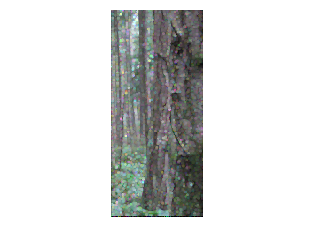
目前修复思路: 由于观察到mask基本都是胡椒噪声(黑色),因此最大值滤波效果会比较好一点,但是仍然会有少量椒盐噪声残余,因此,可以采用将降噪后的图像再次降噪(而不是扩大过滤核大小)。 在这里剩余的仍然是胡椒噪声(黑色),但是经过测试可以看出最大值滤波对图像的影响明显大于中值滤波,最大值滤波会比较模糊,因此这边采用的是“最大值滤波+中值滤波”的组合。(注:为什么先用最大值滤波?因为实验测试第一次就用中值滤波效果很差)
直接使用中值滤波实验结果:
用savefig保存时,图片会有压缩,导致保存和重新从文件中读取的内容有些区别
1
2
3
4
5
6
7
noised_im = NoiseGenerator.add_pulse_noise(im) plt.imshow(noised_im) plt.axis("off" ) plt.savefig("A_noised.png" ) src = "A_noised.png" dst = "A_repaired.png" MedianFilter(src, dst)
samples给的图中噪声基本都是胡椒噪声,没有什么盐噪声,因此考虑最大值滤波
当黑色占比大于0.3时使用"最大值滤波+中值滤波组合", 当小于0.3时直接使用中值滤波
k=5太模糊,目前使用k=3
1 2 3 4 5 6 7 8 9 10 11 12 13 14 15 16 17 18 19 20 21 22 23 24 25 26 27 28 29 30 31 32 33 34 35 36 def add_noise (filename) : im = cv2.imread(filename) cv2.imshow('original img' , im) h, w = im.shape[0 :2 ] pNum = h * w nRate = 0.3 for r in range(int(pNum * nRate)): randh = random.randint(0 , h - 1 ) randw = random.randint(0 , w - 1 ) if random.random() < 0.5 : im[randh, randw, :] = np.array([0 , 0 , 0 ]) else : im[randh, randw, :] = np.array([255 , 255 , 255 ]) cv2.imshow('add noise' , im) cv2.waitKey(0 ) add_noise('A.png' ) def show_photo (pic_path) : """ :param pic_path: 图片路径 :return: <class 'numpy.ndarray'> """ im = cv2.imread(pic_path) im = cv2.cvtColor(im, cv2.COLOR_BGR2RGB) plt.imshow(im) plt.axis('off' ) plt.show() return im
1
2
3
4
5
6
7
8
9
10
11
12
13
14
15
16
17
18
19
20
21
22
23
24
25
26
27
@_preprocess_data(label_namer=None) def imshow (self, X, cmap=None, norm=None, aspect=None, interpolation=None, alpha=None, vmin=None, vmax=None, origin=None, extent=None, shape=None, filternorm=1 , filterrad=4.0 , imlim=None, resample=None, url=None, **kwargs) : """ Display an image on the axes. Parameters ---------- X : array_like, shape (n, m) or (n, m, 3) or (n, m, 4) Display the image in `X` to current axes. `X` may be an array or a PIL image. If `X` is an array, it can have the following shapes and types: - MxN -- values to be mapped (float or int) - MxNx3 -- RGB (float or uint8) - MxNx4 -- RGBA (float or uint8) MxN arrays are mapped to colors based on the `norm` (mapping scalar to scalar) and the `cmap` (mapping the normed scalar to a color). Elements of RGB and RGBA arrays represent pixels of an MxN image. All values should be in the range [0 .. 1] for floats or [0 .. 255] for integers. Out-of-range values will be clipped to these bounds.
1 # Clipping input data to the valid range for imshow with RGB data ([0..1] for floats or [0..255] for integers).
按照上述信息可知,如果元素为float类型且超过了1,则会被clip,这边clip就是上下限幅,而不是截取小数点后部分
1
2
3
4
res = np.array([ [[1.22 ,2.22 ,3.22 ]], [[-0.55 ,-0.44 ,-6.55 ]] ]
这是一种全参考的图像质量评价指标,分别从亮度、对比度、结构三个方面度量图像相似性。SSIM取值范围[0, 1],值越大,表示图像失真越小。
把图片表示成一个向量,通过计算向量之间的余弦距离来表征两张图片的相似度。
https://blog.csdn.net/u010977034/article/details/82733137